CFD Calculation Options

To run the calculations, click on the Update calculated data tool. If a problem is found with the grid generation, the CFD Grid Statistics dialog is displayed showing the error. There are three possible error conditions:

1. Maximum cell aspect ratio exceeds the limit - you will need to delete the existing project and create a new one either reducing the default grid spacing dimension or increasing the grid line merge tolerance by a suitable amount (see the CFD Analysis Manager section).
2. Required memory exceeds the available memory - you will need to delete the existing project and create a new project with larger default grid spacing or consider simplifying the problem definition in terms of complexity of assemblies, etc.
3. Flow imbalance – the total flow rate specified for supply diffusers does not balance with the total flow rate specified for extract grilles. You will need to add supply diffusers or extract grilles or edit the existing flow rates to establish the correct balance

If no problem is encountered in creating the grid, the ‘Edit Calculation Options’ dialog will be displayed:

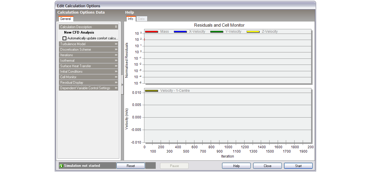
The Edit Calculation Options dialog is divided into two main sections, the Residuals and Cell Monitor graphs and the Calculation Options Data panel. 

Buttons

There are also a group of buttons at the bottom of the dialog, which allow you to control the calculations:

Start

Start, or if the calculations have been paused, re-start the calculations.

Pause

Interrupt or pause the calculations. Once the calculations have been paused, the calculation dialog can be temporarily closed in order to review the results.

Reset

After pausing the calculations, the calculations may then be re-initialised to start from scratch. If the solution is found to diverge and you pause the calculations to decrease the velocity false time steps, you will then need to reset the calculations before re-starting.

The calculation settings panel incorporates the following settings:

Turbulence Model

The following turbulence model options are available:

• 1–Constant effective viscosity: The constant effective viscosity model is a very simple approach involving the replacement of the molecular viscosity in the Navier-Stokes equations with a constant effective viscosity (typically in the order of 100-1000). Although this model is incapable of modelling local turbulence or the transport of turbulence, it is computationally much less expensive than the k-e model and can be numerically much more stable.

• 2–k-e: This model is one of the most widely used and tested of all turbulence models, belonging to the so-called RANS (Reynolds Averaged Navier-Stokes) family of models. These models involve replacing the instantaneous velocity in the Navier-Stokes and energy equations with a mean and fluctuating component. The resulting equations give rise to additional terms known as Reynolds stresses and turbulent heat flux components. Reynolds stresses are replaced with terms involving instantaneous velocities where molecular viscosities are substituted for effective viscosities and a similar substitution is conducted for the energy equation. The effective viscosity is the sum of the molecular viscosity and a turbulent viscosity, which is derived from the turbulence kinetic energy and the dissipation rate of turbulence kinetic energy:

where k= turbulence kinetic energy and  e = dissipation rate of turbulence kinetic energy

k and  e are both derived from partial differential equations which are in turn derived from a manipulation of the Navier-Stokes equations.

Discretisation scheme

The following discretisation schemes are available:

• 1-Upwind - The calculation process involves replacing the defining set of partial differential equations with a set of finite difference equations. The conventional approach to this is to use a Taylor’s series formulation, which leads to a set of central difference equations. However, although this approach is physically realistic for diffusion, it is not found to be realistic for convection because of its one-way nature, i.e. upwind conditions affect downwind conditions but not the reverse. The upwind scheme allows the convective term to be calculated assuming that the value of the dependent variable at a cell interface is equal to the value at the cell on the upwind side of the interface.

• 2–Hybrid – a  more computationally expensive approach than the upwind scheme but it reduces numerical diffusion at high values of Pe number.

• 3–Power-Law - The power-law scheme is arguably more accurate than the hybrid scheme but is more computationally expensive.

Iterations

This is the maximum number of iterations conducted by the outer iterative calculation loop (see ‘CFD Calculations and Convergence’ section). The calculations will terminate when the number of iterations reaches this value regardless of whether or not the solution has converged.

Isothermal

If the Isothermal checkbox is checked the temperature is assumed to be constant throughout the calculation domain and the energy equation is removed from the calculations.

Surface Heat Transfer

Surface heat transfer option

When the Isothermal option is not selected inside surface heat transfer options can be selected from the following 2 options:

• 1–Calculated- Surface heat transfer coefficients are calculated using a wall function if the k-e turbulence model has been selected.

• 2–User-defined- Surface heat transfer coefficients can be specified separately for ceilings, wall and floors (below). The heat transfer is calculated by combining the specified surface transfer coefficient with the cell surface area and the delta T between the surface and the adjacent cell.

Surface Heat Transfer Coefficients

When the 2-User defined surface heat transfer option has been selected, enter the inside convective surface heat transfer coefficients. Coefficients can be entered separately for ceilings, floors and walls.

Ceiling

The ceiling inside surface convective heat transfer coefficient is used in the heat flux calculations between all downward-facing surfaces, including zone ceilings, roofs, and downward facing component block surfaces for component blocks that have the 2-Temperature boundary condition option set. The default user-defined ceiling heat transfer coefficient is 5 W/m2-K.

Wall

The wall inside surface convective heat transfer coefficient is used in the heat flux calculations between all wall and partition surfaces, including zone walls and partitions and non-horizontal component block surfaces for component blocks that have the 2-Temperature boundary condition option set. The default user-defined wall heat transfer coefficient is 2.5 W/m2-K.

Floor

The floor inside surface convective heat transfer coefficient is used in the heat flux calculations between all upward-facing surfaces, including zone floors and upward facing component block surfaces for component blocks that have the 2-Temperature boundary condition option set. The default user-defined floor heat transfer coefficient is 0.7 W/m2-K.

Initial conditions

In some cases, a faster solution can be achieved by setting the initial conditions closer to the final expected conditions. Enter initial velocities in each of the x, y and z directions as well as the initial temperature of the whole domain.

Cell monitor

Select any defined cell monitor point and associated dependent variable to be displayed on the cell monitor (see Setting Up CFD Cell Monitor Points section).

Residual Display

Residuals give an indication of the extent to which the calculations have converged to the final solution. They are a measure of the total 'error' still left on the solution. You can select the dependent variables and/or mass for which residuals are to be displayed in the residuals monitor. The mass residual is similar to the dependent variable residuals but is extracted from a continuity equation mass balance for each cell and is the most significant residual in terms of indicating a successfully converged solution.

The residuals have no units and are normalised by scaling to enable similar termination residual magnitudes for each variable.

See also the Termination residual section below.

It is also important to use monitor points (above) in conjunction with termination residuals because they can provide a more meaningful indication of convergence (i.e. when the values of the dependent variables at the monitor points level out).

Dependent Variable Control Settings

Some CFD models may not converge with default control options and may require some adjustment of settings under the Dependent Variable Control Settings header.

The calculations involve a nested iterative scheme whereby dependent variable equations are solved iteratively within an overall outer iterative loop (see CFD Calculations and Convergence section).  The dependent variable control settings enable control inner iterative dependent variable calculations.

Inner iteration

The number of iterations used for the calculation of the dependent variable.

False time step

The finite difference equation set is formulated in the form of a transient equation set although the calculations are essentially a ‘snap-shot’ in time. The reason for this formulation is that the transient term behaves as a very effective relaxation method, which can slow the change in dependent variables in order to arrive at a more stable solution. The false time step is the time step used in the pseudo-transient term of the dependent variable equation. For forced convection flows, a ‘best-guess’ optimal false time step is automatically calculated for velocities, however for buoyancy driven flows, a default value of 0.2 is used. Reducing the false time step has the effect of slowing down the change in the dependent variable and can be a helpful remedy for unstable solutions.

Relaxation factor

This is used in the ‘text book’ relaxation method, which can be used to allow only a proportion of the calculated value of the current iteration dependent variable to be assigned to the variable. However, the false time step is normally the preferred method of achieving under-relaxation.

Termination residual

The outer iterative calculation loop is repeated until the finite difference equations for all cells are satisfied by the current values of the appropriate dependent variables, at which point the scheme is said to have ‘converged’. The dependent variable residual is the maximum residual quantity for the equation balance across all cells in the domain. The solution is deemed to have converged for each dependent variable when the residual is less than the termination residual.

The CFD Calculations and Convergence section gives an overview of the calculation methodology that will help in understanding the concepts used to initialise, control and monitor the calculations.